As you are probably aware Elon Musk has long been wavering in his decision whether or not to purchase Twitter (ticker: TWTR) for a price that would amount to $54.20 a share. For most of the summer it looked like he was going to fight the purchase, and then in early October, claimed he would go ahead with it.

If you look at the stock price of TWTR for the last few months you can see that this has had a stabilizing effect on the price of TWTR during a particular tumultuous market.

If Musk buys TWTR the future price will be certain and not stochastic, this impacts the current price

Notice that after the announcement the stock's price remains relatively stable at a price point just a few dollars below the price point that share holders will receive if Musk purchases the company.

It seems pretty clear here that the market believes that Musk will likely buy Twitter. An interesting probabilistic question to ask is How strongly does the market believe this? That is, can we put a specific probability to the event that Musk will finally purchase Twitter by a specific date?

To answer this question we'll need to take a look at the options market for Twitter. In particularly the Volatility Smile, which is related to the deviation of implied volatility of options in violation of the famous Black-Scholes Merton option pricing model. We'll use both of these tools to construct an empirical Cumulative Distribution Function (CDF) which we can then use to see roughly what probability the market is putting on this acquisition.

A Crash Course in Black-Scholes Merton

To start let's take a look at perhaps the most famous mathematical formula in finance: The Black-Scholes Merton model (BSM model from here on out). This model deserves it's own post, which it will get one day, but for now we need to understand the basic idea.

Despite all of the hype around this model, it basically says we can imagine stocks price movements (viewed in terms of log return, see the Modern Portfolio Theory post for an example) as samples from Geometric Brownian motion. The ending prices of a stock is then just a log-normal distribution, and the expected value of an option (the right to purchase as stock at a fixed price) is just the expectation of the part of that distribution greater (in the case of calls) or lessor (in the case of puts) than the strike price.

The BSM model takes 5 parameters to calculate the price an option:

- $S_0$ current price of the stock

- $K$ the strike price that option grants to stock to be bought or sold for

- $r$ the risk-free interest rate (which we'll be assuming is zero for simplicity)

- $T$ the time to expiration of the option (in fractions of a year)

- $\sigma$ the volatility, or standard deviation in annual log returns

The mathematics of pricing looks a bit intimidating, but in practice it is just doing integration over the expected final price of the stock, and the profits that the owner of the option can expect at the date of expiration. In reality the BSM formula just tells us the expected value of the option at expiration which in turn is the option's price.

Implied Volatility

One of the most important things to understand regarding options pricing is the implied volatility. Here's an image of a typical options chain showing the strike, bid, ask and implied volatility:

Showing the implied volatility of a given option.

Of all the parameters used in the BSM model, only one is not known to us at the time we want to buy an option: the volatility $\sigma$.

The solution to this problem of missing information is to determine "what is the volatility at the current price to make the model make sense?" In this way we can read every pricing of an option as a prediction about how much variance there is going to be in future stock prices.

Probabilities Implied by the BSM model

Central to the price of the option is the probability that it expires in the money (ITM). An option being ITM means that the stock price at expiration is higher than the strike for a call option (right to buy the stock) or lower then the price for a put option (right to sell). Basically if an option expires ITM, the owner of the option will profit.

The probability of this happening is baked into the BSM pricing formula. For a call option the pricing formula is:

$$c = S_0 N(d_1) - Ke^{-rT}N(d_2)$$

Where $N$ is the cumulative normal distribution and $d_1$ and $d_2$ are defined as:

$$d_1 = \frac{\text{ln}(S_0/K) + (r+\sigma^2/2)T}{\sigma\sqrt{T}}$$

$$d_2 = d_1 - \sigma\sqrt{T}$$

While explaining that formula in detail is going to have to wait for another post, the only important thing to take away for this post is that for a call option:

$$P(\text{ITM}_\text{call}) = N(d_2)$$

This means that the probability that the final stock price is greater than the strike price is $N(d_2)$. More useful for us is knowing the inverse, the probability that a the final price is less than $K$ is $1-N(d_2)$.

Fat Tails and All That

Whenever I bring up quantitative finance one of the first critiques I hear is "all those models assume log normal behavior which is not the case! Real life involves fat tails so all these pricing models are wrong!" This has been popularized by the writings of Nassim Taleb and several others (correctly) critiquing modern mathematical finance and common statistical assumptions.

While this is absolutely true, the markets are not ignorant of this. It turns out if you look carefully enough you'll realize that markets do price options assuming non-normal probabilities of future values. That is, traders know that the risks are not log-normal and so do not price options the way BSM implies they should.

The rest of our discussion is going to be see how we can take this market information and turn it into a probability distribution that gives us information regarding what the market believes the price will be at expiration.

Volatility Smiles

According to the BSM model, we should expect the implied volatility to be the same for every strike price. If the movement of stock prices where truly log-normal then the price of each strike price would end up implying the same volatility. However it turns out this is not the case at all. In violation of BSM, implied volatility displays what is referred to as the volatility smile (because it looks like a smile! Though really more often a smirk).

The best way to see this is to plot it. Before diving into TWTR, let's take a look at a more well behaved stock, AMZN. Here we're going to look at the implied volatility of different strike prices of an AMZN option expiring on Nov 18, 2022

The ‘volatility smile’ shows that real pricing disagrees with the BSM model.

What we see here is that implied volatility is much higher at the extremes, and notably higher at the lower extremes that the higher ones. This is not what the BSM would predict but it shows that traders do in fact price "fat tails" into options. While this is not a probability distribution, we can see from this alone that traders believe BSM under-prices the risk in the lower prices (and to an extent the higher ones as well). The fact that this curve spikes up pretty steeply means that traders know there are risks of extreme price drops, reflective of the current economic environment we're in.

Prior to the stock market crash of 1987 volatility smiles mostly didn't exist. Investors trusted in the model over their instincts and the result was a catastrophic crash. It's important to note that this means if in 1987 you were a mathematically savy trader you could have recognized that far out of the money puts where very underpriced given the real risk. Any traders that saw this would have made a lot of money during the crash. However this smile tells us that if, after skimming a few Taleb books, you hope to profit in the same way, you are unlikely to end up as fortunate.

The really exciting thing is that, using only the information we've covered so far, we can come up with an empirical cumulative density function that allows us to make probabilistic claims about the market predictions for this stock.

We'll continue to focus on AMZN and finally return to TWTR for to answer our final question.

Building our CDF

In order to understand the market's beliefs regarding the probabilities of certain prices we can use a similar trick to what we used last time when working with censored data. We didn't now the exact probability for each estimate only that we know something about the probability of values being lower or greater than a certain point.

In this case let's consider a Put option, which is the right to sell a stock a the strike price. For these options to be ITM, we care about the probability that the future stock price is lower than the strike. Conveniently we already discussed the solution to this!

$$P(\text{ITM}_\text{put}) = 1-N(d_2)$$

Or if we're thinking in terms of code:

from scipy.stats import norm

def d_1(s_0, k, r, t, sigma):
    return (np.log(s_0/k) + (r + (sigma**2)/2)*t)/ (sigma*np.sqrt(t))

def d_2(s_0, k, r, t, sigma):
    return d_1(s_0, k, r, t, sigma) - sigma*np.sqrt(t)

def p_itm(s_0, k, r, t, sigma):
    return norm.cdf(d_2(s_0, k, r, t, sigma))

And in our case we just want

1 - p_itm(...)

We'll use implied volatility at each strike for our volatility input and everything else is known (for simplicity we'll assume the risk-free rate is 0.0).

If we plot our 1 - p_itm for each strike price we'll end up build our CDF!

We can iterate over the price and plot this out as see below, along with the theoretical CDF from the BSM model:

Notice the difference at the lower strikes between the theoretical and the empirical.

As we can see the empirical distribution puts significantly more probability density in the tails of this distribution. Fat tails are priced in! For example trader's believe that AMZN dropping to $80/share has roughly a 5% probability of happening where as BSM thinks it has less than 1% chance of occurring.

Now let's see what we can figure out about what the market believes Musk is thinking!

Looking at the CDF for Twitter

Let's start by looking at the volatility smile for Twitter for options expiring on November 4th 2022:

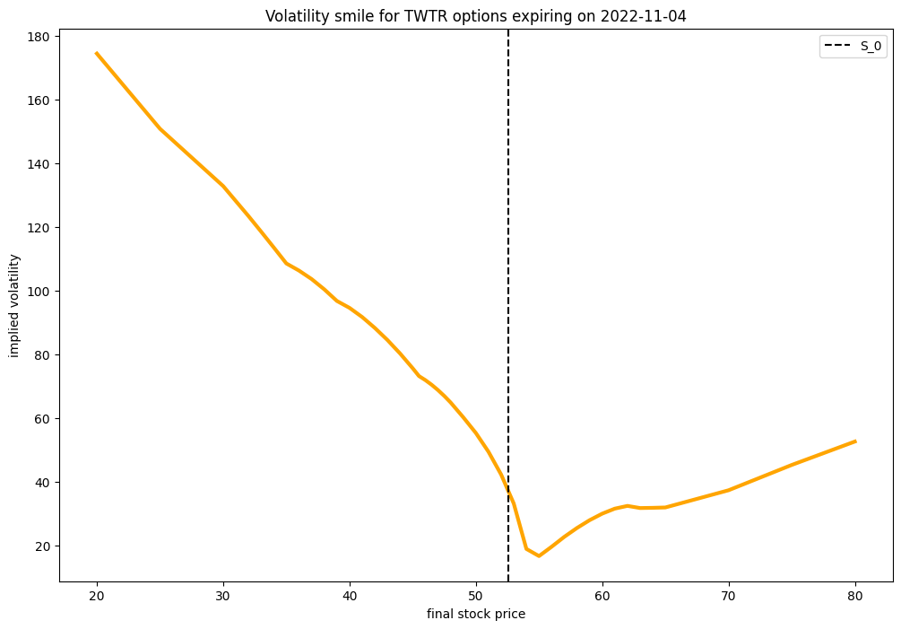
Volatility Smile for Twitter options expiring Nov 4th 2022.

Here we see a much more dramatic and strange smile. It's shaped like a crooked 'v'. It's hard to interpret this in a vacuum so let's look at what this CDF looks like.

Compared to the AMZN CDF this one is much stranger looking!

As expect the empirical distribution looks a lot different from the theoretical, but also a lot different than AMZN!

I've also marked the price per share if Musk completes his purchase in this chart. Looking at AMZN we so a beautiful smooth curve, where as this CDF for TWTR makes a very stark jump from the current price to Musk's price. This is because the market is currently dealing with an interesting statistics question: either TWTR is worth 54.2 per share or ... it's worth something else! The trouble is it's very hard to price TWTR as though Musk hadn't made the offer. So there are really two models hidden here: the Musk price times the probability that Musk does purchase and a distribution of guesses as to what the price might be if he doesn't times the probability he doesn’t purchase.

Thankfully, because of the radical jump, we can make a pretty good estimate as to what the market is predicting. We can look at the range of values where the jump is. I'll say, for ease of estimating, we can focus between the strike of 52 and 55. The probability that TWTR will be less than 52 is currently 0.47 and the probability that it's less than 55 is 0.9. The difference between this two should be our estimate:

$$P(\text{Musk purchases}) = P(S_\text{exp} < 55) - P(S_\text{exp} < 52) = 0.43$$

So, as of this writing, the market believes that there is a 43% chance Musk will go through with the sale by Nov 4th 2022.

What if Musk doesn't go through with the sale

I'm comfortable saying there's a roughly 40% chance that in early November TWTR will be worth exactly 54.2/share to share holders. Suppose you disagree? If you are certain that Musk won’t go through with the sale should you use this opportunity to grab some TWTR stock at a discount?

Clearly the market answer is: No!

In our CDF we can see that only a tiny fraction of the CDF remains above Musk's price, and not very much above it’s current value. Compare this to AMZN which you can see the market believes it could potentially go much higher. Conversely the market has pretty strong beliefs about how low TWTR could go. The probability of TWTR going to 30 or less is currently 0.03. But don't forget that's including the probability that it ends up at the Musk price. This means weighted for the ~60% remaining it's closer to a 5% chance that if Musk does not purchase TWTR it's price will drop to 30.

Conclusion

Quantitative Finance is so fascinating because it is filled with very complex and interesting probability problems that are based on very real world cases. In statistics and data science we often can safely work with well known, and well behaved distributions, even if they aren't a perfect match to our problem. In finance being restricted to models can and has lead to ruin as happened to many adherents to BSM in 1987.

What I find particularly interesting about this case is that even if you have no interest in trading or investing, there is an incredible amount of interesting information contained in the volatility smile. What started my own journey into this particular question was wondering exactly how I could put a number on the probability that Elon Musk will purchase TWTR since it a frequent topic of conversation

By combining statistical tools with a bit of financial engineering thinking we're able to arrive and a very interesting, and reasonable answer to our question. Based on current options prices the market thinks there's a roughly 40% chance Musk will go ahead with this purchase by early November.

Support on Patreon

Support my writing on Patreon and gain access to the source code and video commentary for this article as well as access to much more of my writing!