Using Censored Data to Estimate a Normal Distribution
The other day I received a really interesting inference question from @stevengfan8 on Twitter. Here is the text of the original question:
Suppose you are trying to predict the temperature on a future day. You have an initial prediction of N(75, 5). You ask 10 scientists what their predictions are. The question you pose to each scientist is of the format “Do you think the temperature will be above or below 78 (this can be any number that is not 75)?” You also have historical predictions in this same framework from past days from the same group of scientists and can assume that not every scientist has the same level of predictive skill. How do you incorporate the binary predictions from the scientists into your probabilistic prediction? I’ve been scribbling in a notebook for three hours and haven’t been able to arrive at a reasonable solution
There's a lot to pick apart in this question but we'll focus on the main issue which is:
“How can we estimate a normal distribution around the future date’s temperature only by asking scientists to answer whether or not they believe the temperature will be lower or higher than a specific value?”
This is a very interesting problem and one that is quite relevant to day-to-day statistics. We are often working with nicely defined probability distributions in our models, but it's not always easy to get data that fits these models as nicely. Being limited to asking “yes or no” type questions like this when what we want is numbers is not uncommon.
Let's clarify which parts of this problem we will be ignoring to start with:
- We won't worry about the prior of N(75, 5), though we will use this as our initial guess
- We won't model the not every scientist has the same level of predictive skill
We are just going to start with the problem of modeling the scientists answers to our questions, with the aim of coming up with a normal distribution representing our beliefs about the future temperature.

Surreal scientists contemplating the weather
Simulating our problem
To make sure we have a good grasp on the problem at hand let's simulate our scientists to make sure that whatever solution we propose actually works (at least, in theory). To start with we'll define a true \(\mu\) and \(\sigma\) of our temperature in the future:
MU = 82
SIGMA = 3
Next we'll come up with the questions we will ask the scientists, we'll ask questions from a uniform range of numbers from 65-95, assuming this is roughly what we expect the range of realistic temperatures to be, but assuming that they are all equally likely as far as we know. We'll also specify the number of scientists in our simulation. The original question asks for only 10, but we'll start with 100 just to give our simulation a better chance of being successful.
# Number of scientists we are questioning
N_SCI = 100


# We'll ask them about these thresholds
rng = np.random.default_rng(1337)
sci_questions = rng.uniform(65,95,N_SCI)
We have our questions for the scientists, now we need to model how they'll answer. For this first pass we'll assume that all scientists know the true mean (it turns out that this will give us no way to estimate variance, but we’ll solve this after!). This is the "happy case", after we establish a solution given this situation we can test our model using more uncertainty in the scientists’ individual beliefs.
We'll be representing "greater" as True and "less than" as False.
# We'll start by assuming they're all correct
# True = above, False = below
sci_direction = sci_questions < MU
Placing the questions where they lay on the true distribution with arrows indicating the answers of our scientists can help to give us a view what we're trying to estimate:
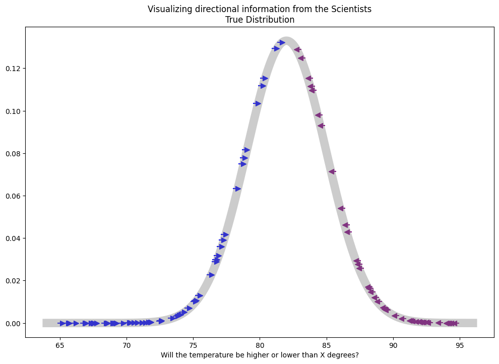
Visually we start to get a clue how we might use these direction answers to estimate our parameters.
Here we can see that when mapped against the true distribution all the arrows point towards the mean. Let’s see what happens when we don’t know the true distribution.
Suppose we use N(75,5) as our initial guess.
mu_est = 75.0
sigma_est = 5
We can produce the same plot with our initial estimated distribution and get a sense of where the error in our model is:

Our answers map to our initial estimates show us that we should move our estimated mean.
What becomes visually obvious here is that there are too many directional answers pointing away from our the mean of our proposed distribution. Visually we can see the data suggest "move to the right!", but we need to figure out how to model this mathematically.
Directional answers and Censored Data
To start understanding our problem mathematically let's consider an easier version of this problem. Suppose instead of asking our scientists about a number we chose, what if we instead asked them for their estimate directly?
In this case it's pretty clear we could just find the normal distribution whose Probability Density Function (PDF) was most consistent with our scientists’ response. In fact we can do this quite easily be simply averaging over the data given to us by the scientists.
The trouble here is we only know the upper and lower bounds of the beliefs of our scientists. Because we're the ones asking the scientist about a number we chose that number itself doesn't give us much information.
This is a type of censored data similar to what we might find in survival analysis problems. In survival analysis we are often concerned with estimating the impact of a treatment given how long patients survive after receiving the treatment. However what do we do when patients don't die at the end of the study (which hopefully they don’t!)?
If we know that a patient survived for 8 years after treatment, but then the trial ended, this seems like very useful information. The patient survived a long time, but they might have survived longer. We can’t use the time they survived until as our data, but we can use the fact that they survived at least that long.
What we need to do now is switch up our thinking so we can estimate beliefs based on censored data.
Making use of the Cumulative Distribution Function
The key issue is that typically when we solve an estimation problem we have a bunch of observed points and we use the PDF of our model distribution to determine the most likely set of parameters that match our data. Here we have ranges of possible values, so we can't use the PDF but we can make use of the Cumulative Distribution Function (CDF).
We need a likelihood function \(P(D|H)\) where D is our data (i.e. the response from the scientists) and H is our hypothesis (i.e. the estimated \(\mu\) and \(\sigma\) for our distribution). To build this function, we'll use \(\Phi(x; \mu, \sigma)\) to represent the cumulative normal distribution function. That is "the probability that a value is less than or equal to x". Given this we can solve our problem as a probability problem like this:

What this formula is telling us is that if the scientist replies the value is lower than x, we take into account that probability, given a set of parameters, that the value is less than x. If they scientist replies that the value is higher we given the probability that the value is higher using 1 - the CDF at x given the parameters.
So our likelihood will be:
$$\Pi_i^N P(x_i; \mu, \sigma)$$
Visually explaining “why the CDF?”
We can understand this better if we plot out a single example comparing the known parameters with our initial estimates. Recall that the CDF is just the integral of the PDF up to a given value, so we can visualize this by shading the area under the curve.
We are using 76.81 as a proposed temperature. The area shaded represents \(1-\Phi(76.81,\mu,\sigma)\) for the case of the known distribution as well as the case of our initial estimate. Because 76.81 is censored we only know that the temperature will be above this. We can then compare the probability of being greater than 76.81 given each parameterization.

Comparing the observation that “the temperature will greater that 78.6” given two different parameterizations for our model.
As we can see the estimate with the known true parameters is much higher than for our initial estimate.
For the case of a claim that the future temperature will be lower, we would look at the area under the curve for the other direction (which is just the CDF at that value). Here is an visualization of the case where the scientist claims that the value will be lower than the one asked about, in this case 83.61.
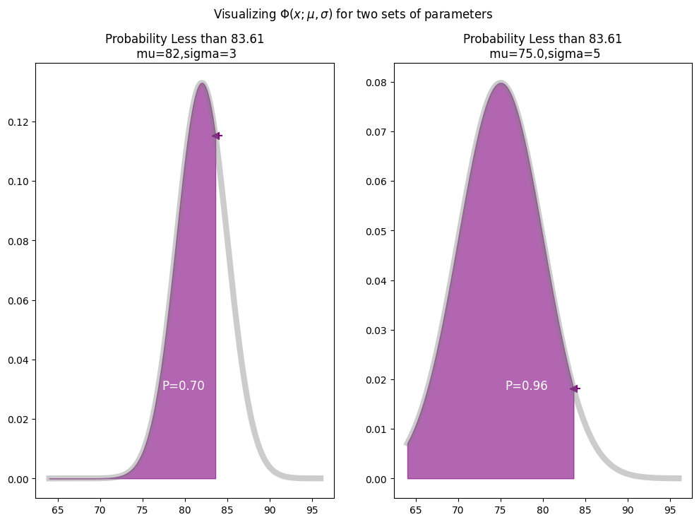
Here we use the regular CDF which is the equivalent of integrating the PDF to the specified value.
In this case we can see that our initial estimate of parameters explains the data a bit better than the true set of parameters.
To compute our likelihood we do this comparison for each observation, calculate he probability of all these observations combined and use it to determine the optimal parameters. In this case of just these two observations and two hypothesis we would have:
$$P(D|H_\text{true}) = 0.96 \cdot 0.7 = 0.672$$
$$P(D|H_\text{est}) = 0.36 \cdot 0.96 = 0.346$$
Which would have our likelihood ratio close to 2, meaning the true parameters explain the data nearly twice as well as the initial estimate for the parameters. In practice we will use all of our data, and of course consider an infinite range of possible parameters for the model, and we’ll use an optimization algorithm to search for these for us.
All we have to do now is write up the code to do this optimization for the most likely \(\mu\) and \(\sigma\) given our data.
Coding up our solution
We'll start by translating what we have here into Python giving us our likelihood:
def likelihood(params, questions, direction):
    mu = params[0]
    sigma = params[1]
    return np.prod(np.where(direction,
                    1-norm.cdf(questions,mu,sigma),
                    norm.cdf(questions,mu,sigma)))
Before going further it's always a good idea to make sure that our function makes sense. We can do this by comparing our initial estimated parameters to the known true parameters (the latter should be much more likely).
> likelihood([mu_est, sigma_est], sci_questions, sci_direction)
1.0272853911142369e-15

> likelihood([MU, SIGMA], sci_questions, sci_direction)
0.0015714199558271044
Looks good to me! Typically we end up optimizing our negative log-likelihood, which is useful because often our optimizers are trying to minimize a value and using the log will dramatically reduce our chance of having overflow problems:
def log_likelihood(params, questions, direction):
    mu = params[0]
    sigma = params[1]
    return np.sum(np.where(direction,
                    np.log(1-norm.cdf(questions,mu,sigma)),
                    np.log(norm.cdf(questions,mu,sigma))))

def neg_log_likelihood(params, questions, direction):
    return - log_likelihood(params, questions, direction)
And we'll do a quick sanity check...
# should be the same as our previous answer
> np.exp(log_likelihood([MU, SIGMA], sci_questions, sci_direction))
0.0015714199558271036
Okay! From here we can just go ahead and use Scipy's minimize to see if we can learn a good estimate.
from scipy.optimize import minimize, Bounds

res = minimize(
    neg_log_likelihood,
    x0=(mu_est,sigma_est),
    args=(sci_questions, sci_direction),
    bounds=Bounds(0.1)
)

> print(res['x'])

"[82.2009337, 0.1]"
Let’s also see what our estimated distribution looks like:

We got the mean perfect, but our variances seems way off (that’s a problem with our simulation, not the model itself)
We can immediately see that while our model is awesome at determining the true value of MU, it is not so great at estimating the value for SIGMA.
This is not to surprising since we didn't model our scientists having variance in their own beliefs across the population. That is there's no variance in their hidden beliefs so we shouldn't expect it to show up here. Let's go ahead and add that variance in, and ultimately model a more realistic version of this problem. After all we would expect that each scientist does have a different opinion of what the true temperature will be in the future.
Modeling more Realistic Scientists
The big reason that our model failed to learn the variance is because the variance never comes into play in our data!
All of our scientists shared the exact same belief in the underlying data, that is they all agreed upon the true MU for the data. This time when we update the scientist direction we won't measure it in terms of the True MU but rather a value sampled from N(MU, SIGMA).
Here's the code for our new data.
# now each individual scientist has their own internal belief about the
# true mean.
sci_mu = rng.normal(MU, SIGMA, N_SCI)

# note that the questions have not changed.
sci_direction_uncertain = sci_questions < sci_mu
Plotting this out we can see there are a few scientists who are on the wrong side of the true distribution because their beliefs now differ from the others.

As we can see, we know have variance in beliefs, and not all of them point towards the true mean.
Now we can optimize our estimates with this new data.
res_uncertain = minimize(
                neg_log_likelihood,
                x0=(mu_est,sigma_est),
                args=(sci_questions, sci_direction_uncertain),
                bounds=Bounds(0.1)
)

> print(res_uncertain['x'])
"[81.88805088, 2.32176536]"
Our estimates are now much closer to correct for both parameters, and if we were to increase the number of scientists we would find that the estimates for both \(\mu\) and \(\sigma\) would end up very close to exact.
Here is our final model compared to the true distribution.

Correctly simulating our problem gives us a much better model!
As we can see, even though all of our information was censored, we where still able to come up with a pretty good estimate of the distribution of the scientist collective true beliefs.
Conclusion
The key insight when dealing with censored data when estimating is to switch from using the PDF for our main estimation tool to the CDF. Using the CDF is perfectly aligned with the type of information we have, we only know directional information about our problem.
Two other questions in the original question where how to incorporate a prior belief and how to incorporate the fact that we know some scientists are more reliable than others (which is it’s own type of prior!). The answer to both of these is the same. For the prior we just weigh each value in our distribution by it's prior probability, and likewise if we have a numeric weight for each scientist we can apply this as well.
Dealing with censored data is a problem that comes up frequently in real life but tends to be under discussed. I hope you had fun seeing how we could form a continuous distribution representing the beliefs of our scientists given only their direction answers to our questions! The more I play with this problem the more I think about cases where people can’t give good estimate, but could probably give good direction answers. For example if you wanted to model how many views people believed this post might get, even thought it might be really hard to put an exact number, by simply picking random numbers and asking directional questions you could start to model the populations beliefs about this problem.

Support on Patreon
Support my writing on Patreon and gain access to the source code and video commentary for this article as well as access to much more of my writing!